In this exercise, you will implement a one-layer RICA network and apply them to MNIST images.

You will build on MATLAB starter code which we have provided in the starter code. You need only write code at places indicated by YOUR CODE HERE. You will modify the files softICACost.m and zca2.m

Step 0: Prerequisites

Step 0a: Read runSoftICA.m

The file runSoftICA.m is the “main” script. It handles loading data, preprocessing it, and calling minFunc with the appropriate parameters. Be sure to understand how this file works before moving further.

Step 0b: Implement zca2.m

Implement the ZCA transform in zca2.m. You should be able to copy and paste your code from Exercise: PCA Whitening if you have successfully completed that exercise.

Step 1: RICA cost and gradient

First, let us derive the gradient of the RICA reconstruction cost using the backpropagation idea.

Step 1a: Deriving gradient using Backpropagation

Recall the RICA reconstruction cost term:

\lVert W^TWx - x \rVert_2^2

where W is the weight matrix and x is the input.

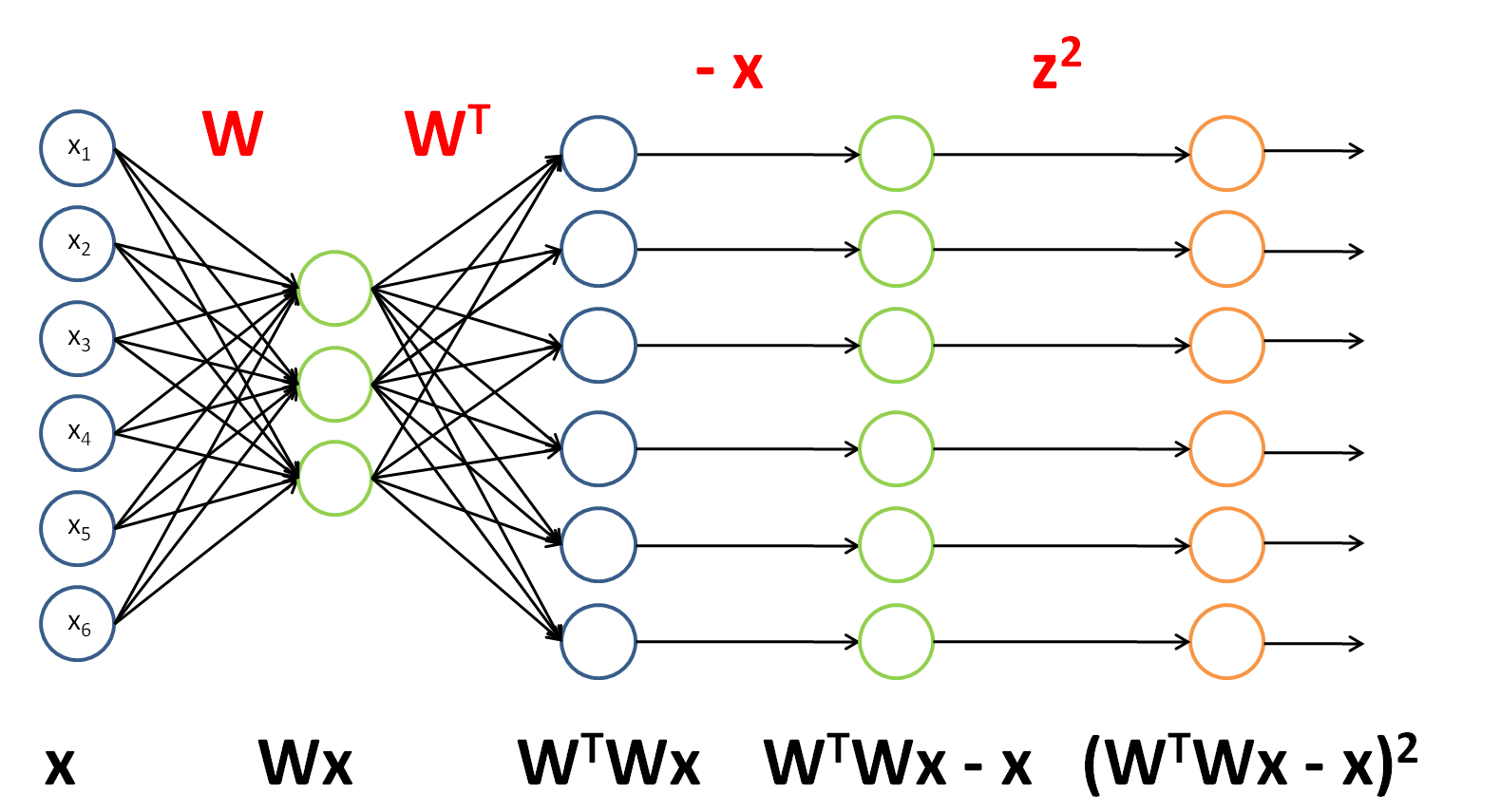
We would like to find \nabla_W \lVert W^TWx - x \rVert_2^2 - the derivative of the term with respect to the ”‘weight matrix”’, rather than the ”‘input”’ as in the earlier two examples. We will still proceed similarly though, seeing this term as an instantiation of a neural network:

The weights and activation functions of this network are as follows:

\text{Layer}	\text{Weight}	\text{Activation function}
1	W	f(z_i) = z_i
2	W^T	f(z_i) = z_i
3	I	f(z_i) = z_i - x_i
4	\text{N/A}	f(z_i) = z_i^2

To have J(z^{(4)}) = F(x), we can set J(z^{(4)}) = \sum_k J(z^{(4)}_k).

Now that we can see F as a neural network, we can try to compute the gradient \nabla_W F. However, we now face the difficulty that W appears twice in the network. Fortunately, it turns out that if W appears multiple times in the network, the gradient with respect to W is simply the sum of gradients for each instance of W in the network (you may wish to work out a formal proof of this fact to convince yourself). With this in mind, we will proceed to work out the deltas first:

\text{Layer}	\text{Derivative of activation function }f'	\text{Delta}	\text{Input }z \text{ to this layer}
4	f'(z_i) = 2z_i	f'(z_i) = 2z_i	(W^TWx - x)
3	f'(z_i) = 1	\left( I^T \delta^{(4)} \right) \bullet 1	W^TWx
2	f'(z_i) = 1	\left( (W^T)^T \delta^{(3)} \right) \bullet 1	Wx
1	f'(z_i) = 1	\left( W^T \delta^{(2)} \right) \bullet 1	x

To find the gradients with respect to W, first we find the gradients with respect to each instance of W in the network.

With respect to W^T:

\begin{align} \nabla_{W^T} F & = \delta^{(3)} a^{(2)T} \\ & = 2(W^TWx - x) (Wx)^T \end{align}

With respect to W:

\begin{align} \nabla_{W} F & = \delta^{(2)} a^{(1)T} \\ & = (W)(2(W^TWx -x)) x^T \end{align}

Taking sums, noting that we need to transpose the gradient with respect to W^T to get the gradient with respect to W, yields the final gradient with respect to W (pardon the slight abuse of notation here):

\begin{align} \nabla_{W} F & = \nabla_{W} F + (\nabla_{W^T} F)^T \\ & = (W)(2(W^TWx -x)) x^T + 2(Wx)(W^TWx - x)^T \end{align}

Step 1b: Implement cost and gradient

In the file softICACost.m, implement the RICA cost and gradient. The cost we use is:

\min_{W} \quad \lambda \left\|Wx\right\|_1 + \frac{1}{2} \left\| W^T Wx - x \right\|_2^2

Note that this is slightly different than the cost used in the gradient derivation section above (because we have added the L1 regularization and scaled the reconstruction term down by 0.5). To implement the L1-norm, we suggest using: f(x) = \sqrt{x^2 + \epsilon} for some small \epsilon. In this exercise, we find \epsilon=0.01 to work well.

When done, check your gradient implementation. You could do this either using your own checkNumericalGradient.m from previous sections, or by using minFunc’s built-in checker.

Comparison Results

TODO