Introduction

Principal Components Analysis (PCA) is a dimensionality reduction algorithm that can be used to significantly speed up your unsupervised feature learning algorithm. More importantly, understanding PCA will enable us to later implement whitening, which is an important pre-processing step for many algorithms.

Suppose you are training your algorithm on images. Then the input will be somewhat redundant, because the values of adjacent pixels in an image are highly correlated. Concretely, suppose we are training on 16x16 grayscale image patches. Then \textstyle x \in \Re^{256} are 256 dimensional vectors, with one feature \textstyle x_j corresponding to the intensity of each pixel. Because of the correlation between adjacent pixels, PCA will allow us to approximate the input with a much lower dimensional one, while incurring very little error.

Example and Mathematical Background

For our running example, we will use a dataset \textstyle \{x^{(1)}, x^{(2)}, \ldots, x^{(m)}\} with \textstyle n=2 dimensional inputs, so that \textstyle x^{(i)} \in \Re^2. Suppose we want to reduce the data from 2 dimensions to 1. (In practice, we might want to reduce data from 256 to 50 dimensions, say; but using lower dimensional data in our example allows us to visualize the algorithms better.) Here is our dataset:

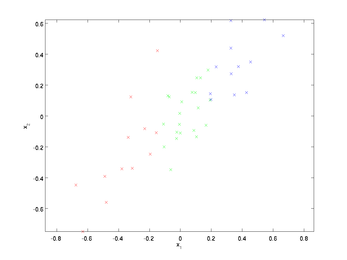
This data has already been pre-processed so that each of the features \textstyle x_1 and \textstyle x_2 have about the same mean (zero) and variance.

For the purpose of illustration, we have also colored each of the points one of three colors, depending on their \textstyle x_1 value; these colors are not used by the algorithm, and are for illustration only.

PCA will find a lower-dimensional subspace onto which to project our data.
From visually examining the data, it appears that \textstyle u_1 is the principal direction of variation of the data, and \textstyle u_2 the secondary direction of variation:

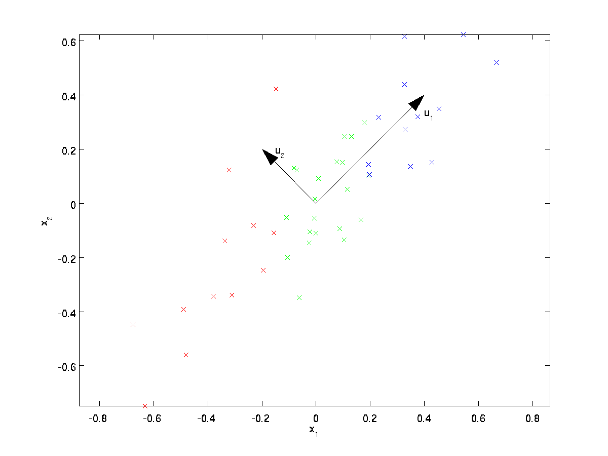
I.e., the data varies much more in the direction \textstyle u_1 than \textstyle u_2. To more formally find the directions \textstyle u_1 and \textstyle u_2, we first compute the matrix \textstyle \Sigma as follows:

If \textstyle x has zero mean, then \textstyle \Sigma is exactly the covariance matrix of \textstyle x. (The symbol ”\textstyle \Sigma”, pronounced “Sigma”, is the standard notation for denoting the covariance matrix. Unfortunately it looks just like the summation symbol, as in \sum_{i=1}^n i; but these are two different things.)

It can then be shown that \textstyle u_1—the principal direction of variation of the data—is the top (principal) eigenvector of \textstyle \Sigma, and \textstyle u_2 is the second eigenvector.

Note: If you are interested in seeing a more formal mathematical derivation/justification of this result, see the CS229 (Machine Learning) lecture notes on PCA (link at bottom of this page). You won’t need to do so to follow along this course, however.

You can use standard numerical linear algebra software to find these eigenvectors (see Implementation Notes). Concretely, let us compute the eigenvectors of \textstyle \Sigma, and stack the eigenvectors in columns to form the matrix \textstyle U:

Here, \textstyle u_1 is the principal eigenvector (corresponding to the largest eigenvalue), \textstyle u_2 is the second eigenvector, and so on. Also, let \textstyle \lambda_1, \lambda_2, \ldots, \lambda_n be the corresponding eigenvalues.

The vectors \textstyle u_1 and \textstyle u_2 in our example form a new basis in which we can represent the data. Concretely, let \textstyle x \in \Re^2 be some training example. Then \textstyle u_1^Tx is the length (magnitude) of the projection of \textstyle x onto the vector \textstyle u_1.

Similarly, \textstyle u_2^Tx is the magnitude of \textstyle x projected onto the vector \textstyle u_2.

Rotating the Data

Thus, we can represent \textstyle x in the \textstyle (u_1, u_2)-basis by computing

(The subscript “rot” comes from the observation that this corresponds to a rotation (and possibly reflection) of the original data.) Lets take the entire training set, and compute \textstyle x_{\rm rot}^{(i)} = U^Tx^{(i)} for every \textstyle i. Plotting this transformed data \textstyle x_{\rm rot}, we get:

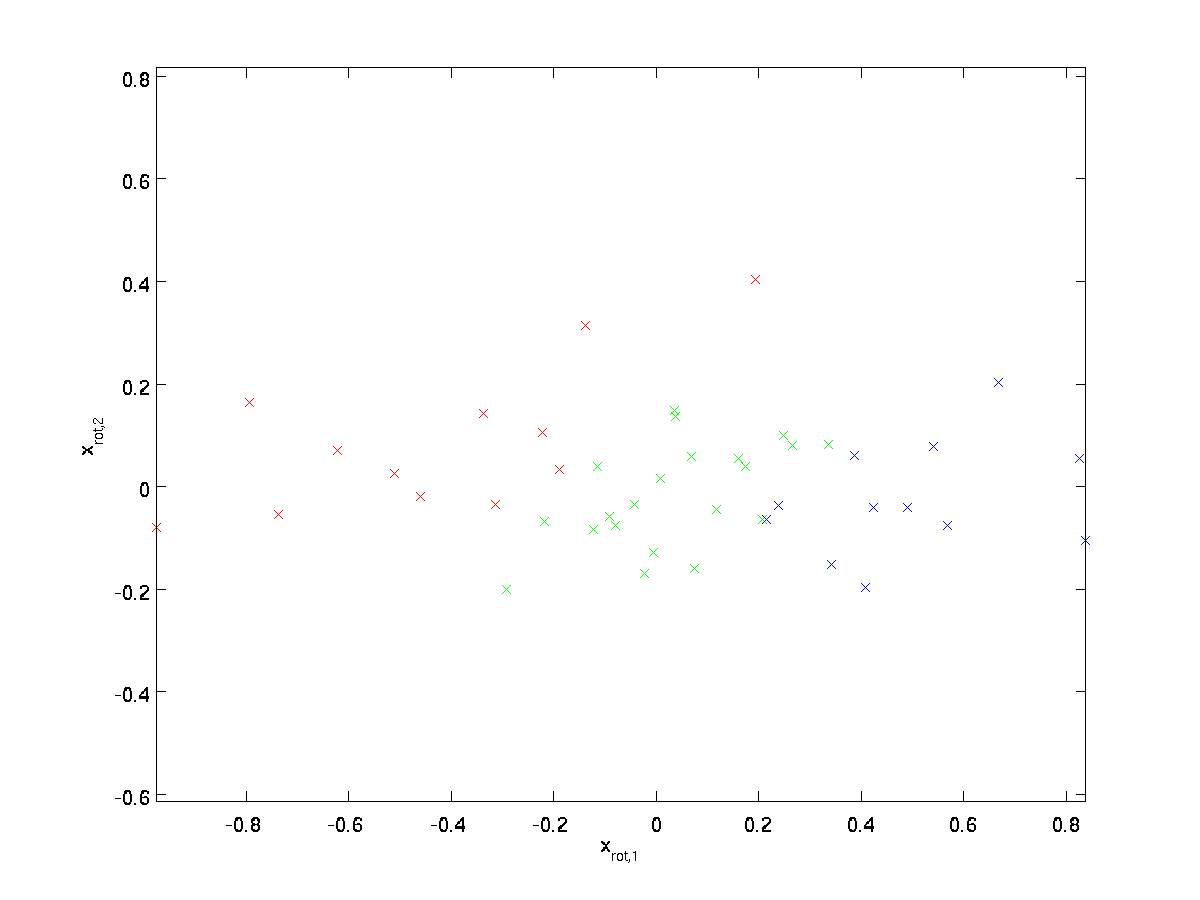
This is the training set rotated into the \textstyle u_1,\textstyle u_2 basis. In the general case, \textstyle U^Tx will be the training set rotated into the basis \textstyle u_1,\textstyle u_2, …,\textstyle u_n.

One of the properties of \textstyle U is that it is an “orthogonal” matrix, which means that it satisfies \textstyle U^TU = UU^T = I. So if you ever need to go from the rotated vectors \textstyle x_{\rm rot} back to the original data \textstyle x, you can compute

because \textstyle U x_{\rm rot} = UU^T x = x.

Reducing the Data Dimension

We see that the principal direction of variation of the data is the first dimension \textstyle x_{\rm rot,1} of this rotated data. Thus, if we want to reduce this data to one dimension, we can set

More generally, if \textstyle x \in \Re^n and we want to reduce it to a \textstyle k dimensional representation \textstyle \tilde{x} \in \Re^k (where k < n), we would take the first \textstyle k components of \textstyle x_{\rm rot}, which correspond to the top \textstyle k directions of variation.

Another way of explaining PCA is that \textstyle x_{\rm rot} is an \textstyle n dimensional vector, where the first few components are likely to be large (e.g., in our example, we saw that \textstyle x_{\rm rot,1}^{(i)} = u_1^Tx^{(i)} takes reasonably large values for most examples \textstyle i), and the later components are likely to be small (e.g., in our example, \textstyle x_{\rm rot,2}^{(i)} = u_2^Tx^{(i)} was more likely to be small). What PCA does it it drops the the later (smaller) components of \textstyle x_{\rm rot}, and just approximates them with 0’s. Concretely, our definition of \textstyle \tilde{x} can also be arrived at by using an approximation to \textstyle x_{\rm rot} where all but the first \textstyle k components are zeros. In other words, we have:

In our example, this gives us the following plot of \textstyle \tilde{x} (using \textstyle n=2, k=1):

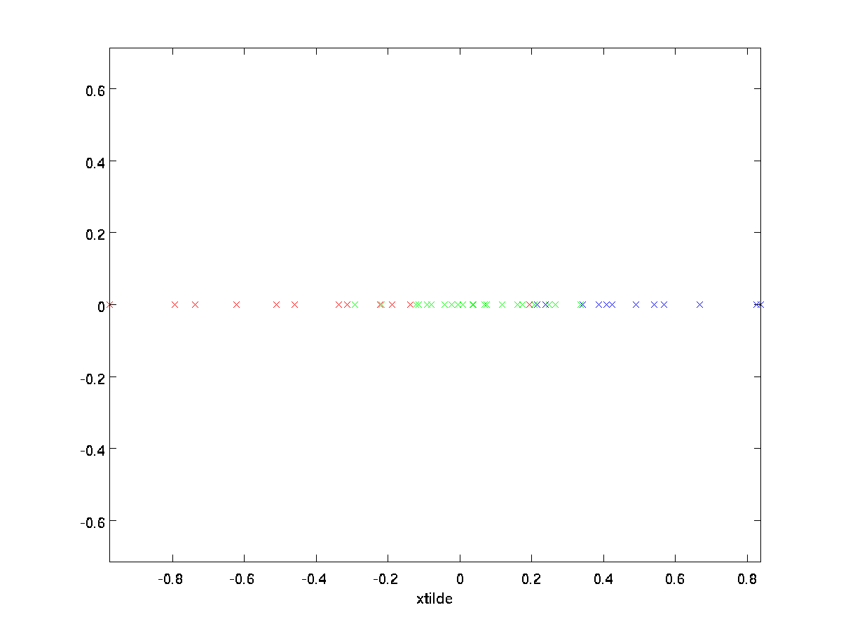
However, since the final \textstyle n-k components of \textstyle \tilde{x} as defined above would always be zero, there is no need to keep these zeros around, and so we define \textstyle \tilde{x} as a \textstyle k-dimensional vector with just the first \textstyle k (non-zero) components.

This also explains why we wanted to express our data in the \textstyle u_1, u_2, \ldots, u_n basis: Deciding which components to keep becomes just keeping the top \textstyle k components. When we do this, we also say that we are “retaining the top \textstyle k PCA (or principal) components.”

Recovering an Approximation of the Data

Now, \textstyle \tilde{x} \in \Re^k is a lower-dimensional, “compressed” representation of the original \textstyle x \in \Re^n. Given \textstyle \tilde{x}, how can we recover an approximation \textstyle \hat{x} to the original value of \textstyle x? From an earlier section, we know that \textstyle x = U x_{\rm rot}. Further, we can think of \textstyle \tilde{x} as an approximation to \textstyle x_{\rm rot}, where we have set the last \textstyle n-k components to zeros. Thus, given \textstyle \tilde{x} \in \Re^k, we can pad it out with \textstyle n-k zeros to get our approximation to \textstyle x_{\rm rot} \in \Re^n. Finally, we pre-multiply by \textstyle U to get our approximation to \textstyle x. Concretely, we get

The final equality above comes from the definition of \textstyle U given earlier. (In a practical implementation, we wouldn’t actually zero pad \textstyle \tilde{x} and then multiply by \textstyle U, since that would mean multiplying a lot of things by zeros; instead, we’d just multiply \textstyle \tilde{x} \in \Re^k with the first \textstyle k columns of \textstyle U as in the final expression above.) Applying this to our dataset, we get the following plot for \textstyle \hat{x}:

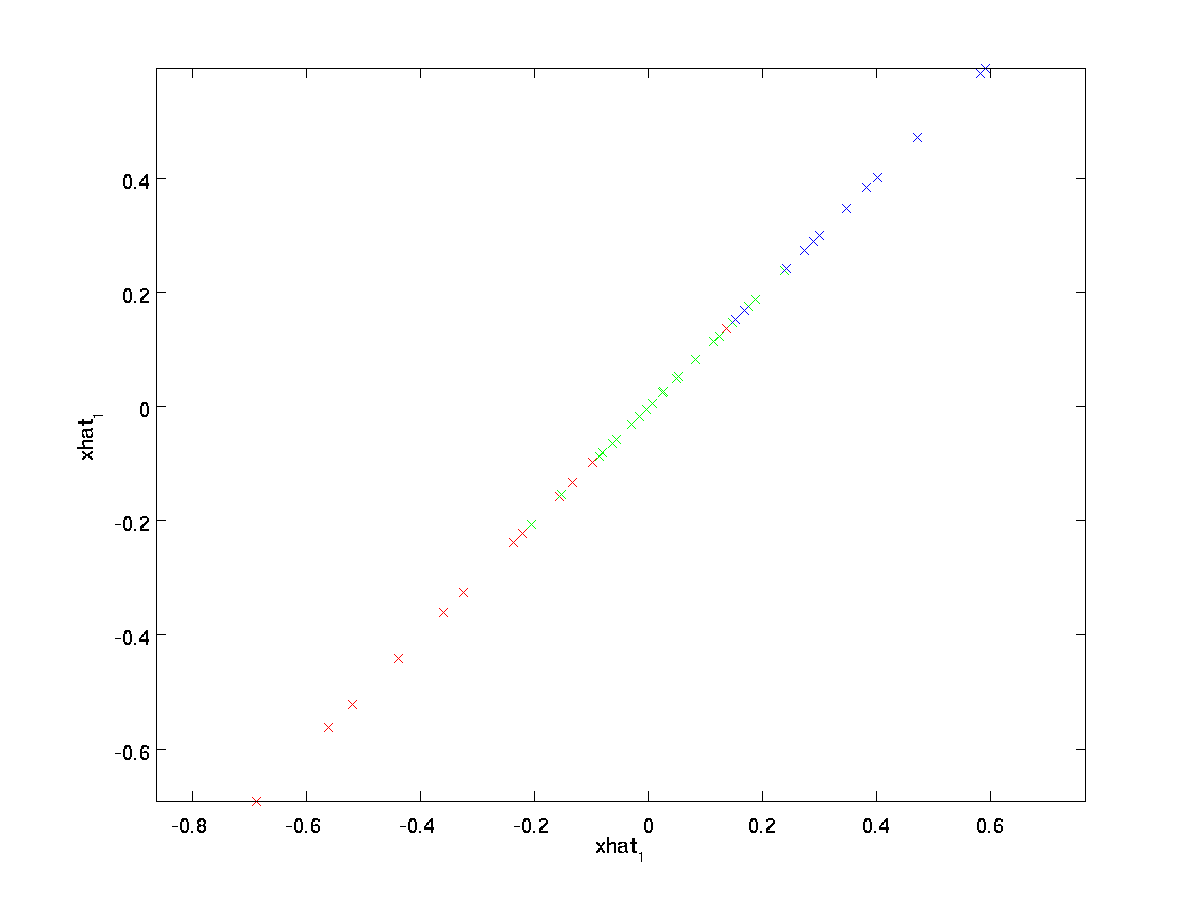
We are thus using a 1 dimensional approximation to the original dataset.

If you are training an autoencoder or other unsupervised feature learning algorithm, the running time of your algorithm will depend on the dimension of the input. If you feed \textstyle \tilde{x} \in \Re^k into your learning algorithm instead of \textstyle x, then you’ll be training on a lower-dimensional input, and thus your algorithm might run significantly faster. For many datasets, the lower dimensional \textstyle \tilde{x} representation can be an extremely good approximation to the original, and using PCA this way can significantly speed up your algorithm while introducing very little approximation error.

Number of components to retain

How do we set \textstyle k; i.e., how many PCA components should we retain? In our simple 2 dimensional example, it seemed natural to retain 1 out of the 2 components, but for higher dimensional data, this decision is less trivial. If \textstyle k is too large, then we won’t be compressing the data much; in the limit of \textstyle k=n, then we’re just using the original data (but rotated into a different basis). Conversely, if \textstyle k is too small, then we might be using a very bad approximation to the data.

To decide how to set \textstyle k, we will usually look at the ”‘percentage of variance retained”’ for different values of \textstyle k. Concretely, if \textstyle k=n, then we have an exact approximation to the data, and we say that 100% of the variance is retained. I.e., all of the variation of the original data is retained. Conversely, if \textstyle k=0, then we are approximating all the data with the zero vector, and thus 0% of the variance is retained.

More generally, let \textstyle \lambda_1, \lambda_2, \ldots, \lambda_n be the eigenvalues of \textstyle \Sigma (sorted in decreasing order), so that \textstyle \lambda_j is the eigenvalue corresponding to the eigenvector \textstyle u_j. Then if we retain \textstyle k principal components, the percentage of variance retained is given by:

In our simple 2D example above, \textstyle \lambda_1 = 7.29, and \textstyle \lambda_2 = 0.69. Thus, by keeping only \textstyle k=1 principal components, we retained \textstyle 7.29/(7.29+0.69) = 0.913, or 91.3% of the variance.

A more formal definition of percentage of variance retained is beyond the scope of these notes. However, it is possible to show that \textstyle \lambda_j = \sum_{i=1}^m x_{\rm rot,j}^2. Thus, if \textstyle \lambda_j \approx 0, that shows that \textstyle x_{\rm rot,j} is usually near 0 anyway, and we lose relatively little by approximating it with a constant 0. This also explains why we retain the top principal components (corresponding to the larger values of \textstyle \lambda_j) instead of the bottom ones. The top principal components \textstyle x_{\rm rot,j} are the ones that’re more variable and that take on larger values, and for which we would incur a greater approximation error if we were to set them to zero.

In the case of images, one common heuristic is to choose \textstyle k so as to retain 99% of the variance. In other words, we pick the smallest value of \textstyle k that satisfies

Depending on the application, if you are willing to incur some additional error, values in the 90-98% range are also sometimes used. When you describe to others how you applied PCA, saying that you chose \textstyle k to retain 95% of the variance will also be a much more easily interpretable description than saying that you retained 120 (or whatever other number of) components.

PCA on Images

For PCA to work, usually we want each of the features \textstyle x_1, x_2, \ldots, x_n to have a similar range of values to the others (and to have a mean close to zero). If you’ve used PCA on other applications before, you may therefore have separately pre-processed each feature to have zero mean and unit variance, by separately estimating the mean and variance of each feature \textstyle x_j. However, this isn’t the pre-processing that we will apply to most types of images. Specifically, suppose we are training our algorithm on ”‘natural images”’, so that \textstyle x_j is the value of pixel \textstyle j. By “natural images,” we informally mean the type of image that a typical animal or person might see over their lifetime.

Note: Usually we use images of outdoor scenes with grass, trees, etc., and cut out small (say 16x16) image patches randomly from these to train the algorithm. But in practice most feature learning algorithms are extremely robust to the exact type of image it is trained on, so most images taken with a normal camera, so long as they aren’t excessively blurry or have strange artifacts, should work.

When training on natural images, it makes little sense to estimate a separate mean and variance for each pixel, because the statistics in one part of the image should (theoretically) be the same as any other.
This property of images is called ”‘stationarity.”’

In detail, in order for PCA to work well, informally we require that (i) The features have approximately zero mean, and (ii) The different features have similar variances to each other. With natural images, (ii) is already satisfied even without variance normalization, and so we won’t perform any variance normalization.
(If you are training on audio data—say, on spectrograms—or on text data—say, bag-of-word vectors—we will usually not perform variance normalization either.)
In fact, PCA is invariant to the scaling of the data, and will return the same eigenvectors regardless of the scaling of the input. More formally, if you multiply each feature vector \textstyle x by some positive number (thus scaling every feature in every training example by the same number), PCA’s output eigenvectors will not change.

So, we won’t use variance normalization. The only normalization we need to perform then is mean normalization, to ensure that the features have a mean around zero. Depending on the application, very often we are not interested in how bright the overall input image is. For example, in object recognition tasks, the overall brightness of the image doesn’t affect what objects there are in the image. More formally, we are not interested in the mean intensity value of an image patch; thus, we can subtract out this value, as a form of mean normalization.

Concretely, if \textstyle x^{(i)} \in \Re^{n} are the (grayscale) intensity values of a 16x16 image patch (\textstyle n=256), we might normalize the intensity of each image \textstyle x^{(i)} as follows:

for all \textstyle j

Note that the two steps above are done separately for each image \textstyle x^{(i)}, and that \textstyle \mu^{(i)} here is the mean intensity of the image \textstyle x^{(i)}. In particular, this is not the same thing as estimating a mean value separately for each pixel \textstyle x_j.

If you are training your algorithm on images other than natural images (for example, images of handwritten characters, or images of single isolated objects centered against a white background), other types of normalization might be worth considering, and the best choice may be application dependent. But when training on natural images, using the per-image mean normalization method as given in the equations above would be a reasonable default.

Whitening

We have used PCA to reduce the dimension of the data. There is a closely related preprocessing step called whitening (or, in some other literatures, sphering) which is needed for some algorithms. If we are training on images, the raw input is redundant, since adjacent pixel values are highly correlated. The goal of whitening is to make the input less redundant; more formally, our desiderata are that our learning algorithms sees a training input where (i) the features are less correlated with each other, and (ii) the features all have the same variance.

2D example

We will first describe whitening using our previous 2D example. We will then describe how this can be combined with smoothing, and finally how to combine this with PCA.

How can we make our input features uncorrelated with each other? We had already done this when computing \textstyle x_{\rm rot}^{(i)} = U^Tx^{(i)}.
Repeating our previous figure, our plot for \textstyle x_{\rm rot} was:

The covariance matrix of this data is given by:

(Note: Technically, many of the statements in this section about the “covariance” will be true only if the data has zero mean. In the rest of this section, we will take this assumption as implicit in our statements. However, even if the data’s mean isn’t exactly zero, the intuitions we’re presenting here still hold true, and so this isn’t something that you should worry about.)

It is no accident that the diagonal values are \textstyle \lambda_1 and \textstyle \lambda_2. Further, the off-diagonal entries are zero; thus, \textstyle x_{\rm rot,1} and \textstyle x_{\rm rot,2} are uncorrelated, satisfying one of our desiderata for whitened data (that the features be less correlated).

To make each of our input features have unit variance, we can simply rescale each feature \textstyle x_{\rm rot,i} by \textstyle 1/\sqrt{\lambda_i}. Concretely, we define our whitened data \textstyle x_{\rm PCAwhite} \in \Re^n as follows:

Plotting \textstyle x_{\rm PCAwhite}, we get:

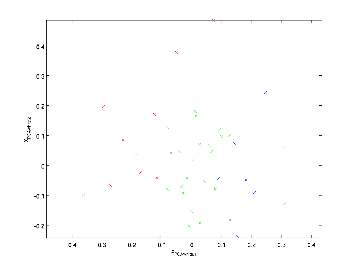
This data now has covariance equal to the identity matrix \textstyle I. We say that \textstyle x_{\rm PCAwhite} is our PCA whitened version of the data: The different components of \textstyle x_{\rm PCAwhite} are uncorrelated and have unit variance.

Whitening combined with dimensionality reduction. If you want to have data that is whitened and which is lower dimensional than the original input, you can also optionally keep only the top \textstyle k components of \textstyle x_{\rm PCAwhite}. When we combine PCA whitening with regularization (described later), the last few components of \textstyle x_{\rm PCAwhite} will be nearly zero anyway, and thus can safely be dropped.

ZCA Whitening

Finally, it turns out that this way of getting the data to have covariance identity \textstyle I isn’t unique. Concretely, if \textstyle R is any orthogonal matrix, so that it satisfies \textstyle RR^T = R^TR = I (less formally, if \textstyle R is a rotation/reflection matrix), then \textstyle R \,x_{\rm PCAwhite} will also have identity covariance.

In ZCA whitening, we choose \textstyle R = U. We define

Plotting \textstyle x_{\rm ZCAwhite}, we get:

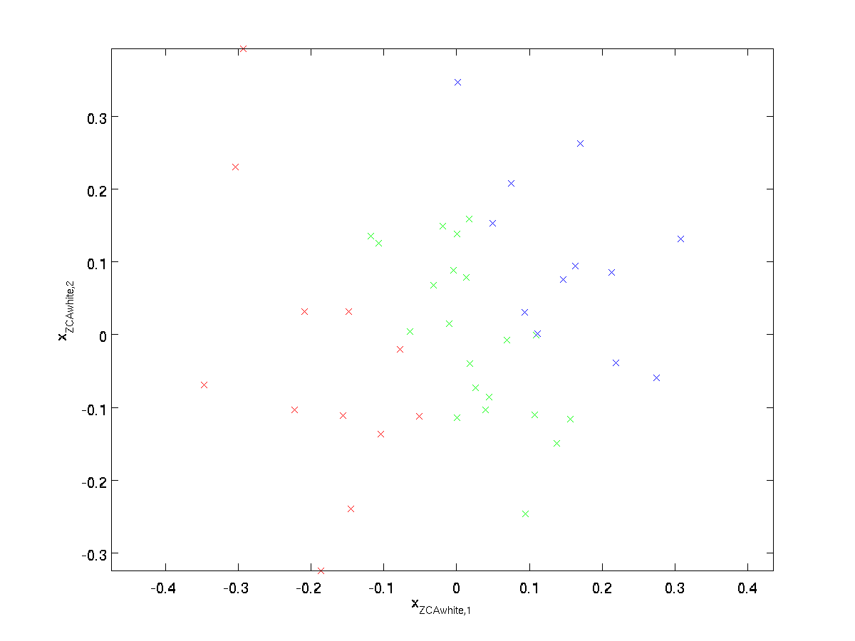
It can be shown that out of all possible choices for \textstyle R, this choice of rotation causes \textstyle x_{\rm ZCAwhite} to be as close as possible to the original input data \textstyle x.

When using ZCA whitening (unlike PCA whitening), we usually keep all \textstyle n dimensions of the data, and do not try to reduce its dimension.

Regularizaton

When implementing PCA whitening or ZCA whitening in practice, sometimes some of the eigenvalues \textstyle \lambda_i will be numerically close to 0, and thus the scaling step where we divide by \sqrt{\lambda_i} would involve dividing by a value close to zero; this may cause the data to blow up (take on large values) or otherwise be numerically unstable. In practice, we therefore implement this scaling step using a small amount of regularization, and add a small constant \textstyle \epsilon to the eigenvalues before taking their square root and inverse:

When \textstyle x takes values around \textstyle [-1,1], a value of \textstyle \epsilon \approx 10^{-5} might be typical.

For the case of images, adding \textstyle \epsilon here also has the effect of slightly smoothing (or low-pass filtering) the input image. This also has a desirable effect of removing aliasing artifacts caused by the way pixels are laid out in an image, and can improve the features learned (details are beyond the scope of these notes).

ZCA whitening is a form of pre-processing of the data that maps it from \textstyle x to \textstyle x_{\rm ZCAwhite}. It turns out that this is also a rough model of how the biological eye (the retina) processes images. Specifically, as your eye perceives images, most adjacent “pixels” in your eye will perceive very similar values, since adjacent parts of an image tend to be highly correlated in intensity. It is thus wasteful for your eye to have to transmit every pixel separately (via your optic nerve) to your brain. Instead, your retina performs a decorrelation operation (this is done via retinal neurons that compute a function called “on center, off surround/off center, on surround”) which is similar to that performed by ZCA. This results in a less redundant representation of the input image, which is then transmitted to your brain.

Implementing PCA Whitening

In this section, we summarize the PCA, PCA whitening and ZCA whitening algorithms, and also describe how you can implement them using efficient linear algebra libraries.

First, we need to ensure that the data has (approximately) zero-mean. For natural images, we achieve this (approximately) by subtracting the mean value of each image patch.

We achieve this by computing the mean for each patch and subtracting it for each patch. In Matlab, we can do this by using

 avg = mean(x, 1);     % Compute the mean pixel intensity value separately for each patch. 
 x = x - repmat(avg, size(x, 1), 1);

Next, we need to compute \textstyle \Sigma = \frac{1}{m} \sum_{i=1}^m (x^{(i)})(x^{(i)})^T. If you’re implementing this in Matlab (or even if you’re implementing this in C++, Java, etc., but have access to an efficient linear algebra library), doing it as an explicit sum is inefficient. Instead, we can compute this in one fell swoop as

 sigma = x * x' / size(x, 2);

(Check the math yourself for correctness.) Here, we assume that x is a data structure that contains one training example per column (so, x is a \textstyle n-by-\textstyle m matrix).

Next, PCA computes the eigenvectors of \Sigma. One could do this using the Matlab eig function. However, because \Sigma is a symmetric positive semi-definite matrix, it is more numerically reliable to do this using the svd function. Concretely, if you implement

 [U,S,V] = svd(sigma);

then the matrix U will contain the eigenvectors of \Sigma (one eigenvector per column, sorted in order from top to bottom eigenvector), and the diagonal entries of the matrix S will contain the corresponding eigenvalues (also sorted in decreasing order). The matrix V will be equal to U, and can be safely ignored.

(Note: The svd function actually computes the singular vectors and singular values of a matrix, which for the special case of a symmetric positive semi-definite matrix—which is all that we’re concerned with here—is equal to its eigenvectors and eigenvalues. A full discussion of singular vectors vs. eigenvectors is beyond the scope of these notes.)

Finally, you can compute \textstyle x_{\rm rot} and \textstyle \tilde{x} as follows:

 xRot = U' * x;          % rotated version of the data. 
 xTilde = U(:,1:k)' * x; % reduced dimension representation of the data, 
                         % where k is the number of eigenvectors to keep

This gives your PCA representation of the data in terms of \textstyle \tilde{x} \in \Re^k. Incidentally, if x is a \textstyle n-by-\textstyle m matrix containing all your training data, this is a vectorized implementation, and the expressions above work too for computing x_{\rm rot} and \tilde{x} for your entire training set all in one go. The resulting x_{\rm rot} and \tilde{x} will have one column corresponding to each training example.

To compute the PCA whitened data \textstyle x_{\rm PCAwhite}, use

 xPCAwhite = diag(1./sqrt(diag(S) + epsilon)) * U' * x;

Since S’s diagonal contains the eigenvalues \textstyle \lambda_i, this turns out to be a compact way of computing \textstyle x_{\rm PCAwhite,i} = \frac{x_{\rm rot,i} }{\sqrt{\lambda_i}} simultaneously for all \textstyle i.

Finally, you can also compute the ZCA whitened data \textstyle x_{\rm ZCAwhite} as:

 xZCAwhite = U * diag(1./sqrt(diag(S) + epsilon)) * U' * x;