Logistic Regression


Previously we learned how to predict continuous-valued quantities (e.g., housing prices) as a linear function of input values (e.g., the size of the house). Sometimes we will instead wish to predict a discrete variable such as predicting whether a grid of pixel intensities represents a “0” digit or a “1” digit. This is a classification problem. Logistic regression is a simple classification algorithm for learning to make such decisions.

In linear regression we tried to predict the value of y^{(i)} for the i‘th example x^{(i)} using a linear function y = h_\theta(x) = \theta^\top x.. This is clearly not a great solution for predicting binary-valued labels \left(y^{(i)} \in \{0,1\}\right). In logistic regression we use a different hypothesis class to try to predict the probability that a given example belongs to the “1” class versus the probability that it belongs to the “0” class. Specifically, we will try to learn a function of the form:

\begin{align} P(y=1|x) &= h_\theta(x) = \frac{1}{1 + \exp(-\theta^\top x)} \equiv \sigma(\theta^\top x),\\ P(y=0|x) &= 1 - P(y=1|x) = 1 - h_\theta(x). \end{align}

The function \sigma(z) \equiv \frac{1}{1 + \exp(-z)} is often called the “sigmoid” or “logistic” function – it is an S-shaped function that “squashes” the value of \theta^\top x into the range [0, 1] so that we may interpret h_\theta(x) as a probability. Our goal is to search for a value of \theta so that the probability P(y=1|x) = h_\theta(x) is large when x belongs to the “1” class and small when x belongs to the “0” class (so that P(y=0|x) is large). For a set of training examples with binary labels \{ (x^{(i)}, y^{(i)}) : i=1,\ldots,m\} the following cost function measures how well a given h_\theta does this:

J(\theta) = - \sum_i \left(y^{(i)} \log( h_\theta(x^{(i)}) ) + (1 - y^{(i)}) \log( 1 - h_\theta(x^{(i)}) ) \right).

Note that only one of the two terms in the summation is non-zero for each training example (depending on whether the label y^{(i)} is 0 or 1). When y^{(i)} = 1 minimizing the cost function means we need to make h_\theta(x^{(i)}) large, and when y^{(i)} = 0 we want to make 1 - h_\theta large as explained above. For a full explanation of logistic regression and how this cost function is derived, see the CS229 Notes on supervised learning.

We now have a cost function that measures how well a given hypothesis h_\theta fits our training data. We can learn to classify our training data by minimizing J(\theta) to find the best choice of \theta. Once we have done so, we can classify a new test point as “1” or “0” by checking which of these two class labels is most probable: if P(y=1|x) > P(y=0|x) then we label the example as a “1”, and “0” otherwise. This is the same as checking whether h_\theta(x) > 0.5.

To minimize J(\theta) we can use the same tools as for linear regression. We need to provide a function that computes J(\theta) and \nabla_\theta J(\theta) for any requested choice of \theta. The derivative of J(\theta) as given above with respect to \theta_j is:

\frac{\partial J(\theta)}{\partial \theta_j} = \sum_i x^{(i)}_j (h_\theta(x^{(i)}) - y^{(i)}).

Written in its vector form, the entire gradient can be expressed as:

\nabla_\theta J(\theta) = \sum_i x^{(i)} (h_\theta(x^{(i)}) - y^{(i)})

This is essentially the same as the gradient for linear regression except that now h_\theta(x) = \sigma(\theta^\top x).

Exercise 1B

Starter code for this exercise is included in the Starter Code GitHub Repo in the ex1/ directory.

In this exercise you will implement the objective function and gradient computations for logistic regression and use your code to learn to classify images of digits from the MNIST dataset as either “0” or “1”. Some examples of these digits are shown below:
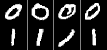
Each of the digits is is represented by a 28x28 grid of pixel intensities, which we will reformat as a vector x^{(i)} with 28*28 = 784 elements. The label is binary, so y^{(i)} \in \{0,1\}.

You will find starter code for this exercise in the ex1/ex1b_logreg.m file. The starter code file performs the following tasks for you:

  1. Calls ex1_load_mnist.m to load the MNIST training and testing data. In addition to loading the pixel values into a matrix X (so that that j’th pixel of the i’th example is X_{ji} = x^{(i)}_j) and the labels into a row-vector y, it will also perform some simple normalizations of the pixel intensities so that they tend to have zero mean and unit variance. Even though the MNIST dataset contains 10 different digits (0-9), in this exercise we will only load the 0 and 1 digits — the ex1_load_mnist function will do this for you.

  2. The code will append a row of 1’s so that \theta_0 will act as an intercept term.

  3. The code calls minFunc with the logistic_regression.m file as objective function. Your job will be to fill in logistic_regression.m to return the objective function value and its gradient.

  4. After minFunc completes, the classification accuracy on the training set and test set will be printed out.

As for the linear regression exercise, you will need to implement logistic_regression.m to loop over all of the training examples x^{(i)} and compute the objective J(\theta; X,y). Store the resulting objective value into the variable f. You must also compute the gradient \nabla_\theta J(\theta; X,y) and store it into the variable g. Once you have completed these tasks, you will be able to run the ex1b_logreg.m script to train the classifier and test it.

If your code is functioning correctly, you should find that your classifier is able to achieve 100% accuracy on both the training and testing sets! It turns out that this is a relatively easy classification problem because 0 and 1 digits tend to look very different. In future exercises it will be much more difficult to get perfect results like this.