Linear Regression


Problem Formulation

As a refresher, we will start by learning how to implement linear regression. The main idea is to get familiar with objective functions, computing their gradients and optimizing the objectives over a set of parameters. These basic tools will form the basis for more sophisticated algorithms later. Readers that want additional details may refer to the Lecture Note on Supervised Learning for more.

Our goal in linear regression is to predict a target value y starting from a vector of input values x \in \Re^n. For example, we might want to make predictions about the price of a house so that y represents the price of the house in dollars and the elements x_j of x represent “features” that describe the house (such as its size and the number of bedrooms). Suppose that we are given many examples of houses where the features for the i’th house are denoted x^{(i)} and the price is y^{(i)}. For short, we will denote the

Our goal is to find a function y = h(x) so that we have y^{(i)} \approx h(x^{(i)}) for each training example. If we succeed in finding a function h(x) like this, and we have seen enough examples of houses and their prices, we hope that the function h(x) will also be a good predictor of the house price even when we are given the features for a new house where the price is not known.

To find a function h(x) where y^{(i)} \approx h(x^{(i)}) we must first decide how to represent the function h(x). To start out we will use linear functions: h_\theta(x) = \sum_j \theta_j x_j = \theta^\top x. Here, h_\theta(x) represents a large family of functions parametrized by the choice of \theta. (We call this space of functions a “hypothesis class”.) With this representation for h, our task is to find a choice of \theta so that h_\theta(x^{(i)}) is as close as possible to y^{(i)}. In particular, we will search for a choice of \theta that minimizes:

J(\theta) = \frac{1}{2} \sum_i \left( h_\theta(x^{(i)}) - y^{(i)} \right)^2 = \frac{1}{2} \sum_i \left( \theta^\top x^{(i)} - y^{(i)} \right)^2

This function is the “cost function” for our problem which measures how much error is incurred in predicting y^{(i)} for a particular choice of \theta. This may also be called a “loss”, “penalty” or “objective” function.

Function Minimization

We now want to find the choice of \theta that minimizes J(\theta) as given above. There are many algorithms for minimizing functions like this one and we will describe some very effective ones that are easy to implement yourself in a later section Gradient descent. For now, let’s take for granted the fact that most commonly-used algorithms for function minimization require us to provide two pieces of information about J(\theta): We will need to write code to compute J(\theta) and \nabla_\theta J(\theta) on demand for any choice of \theta. After that, the rest of the optimization procedure to find the best choice of \theta will be handled by the optimization algorithm. (Recall that the gradient \nabla_\theta J(\theta) of a differentiable function J is a vector that points in the direction of steepest increase as a function of \theta — so it is easy to see how an optimization algorithm could use this to make a small change to \theta that decreases (or increase) J(\theta)).

The above expression for J(\theta) given a training set of x^{(i)} and y^{(i)} is easy to implement in MATLAB to compute J(\theta) for any choice of \theta. The remaining requirement is to compute the gradient:

\nabla_\theta J(\theta) = \begin{align}\left[\begin{array}{c} \frac{\partial J(\theta)}{\partial \theta_1} \\ \frac{\partial J(\theta)}{\partial \theta_2} \\ \vdots\\ \frac{\partial J(\theta)}{\partial \theta_n} \end{array}\right]\end{align}

Differentiating the cost function J(\theta) as given above with respect to a particular parameter \theta_j gives us:

\frac{\partial J(\theta)}{\partial \theta_j} = \sum_i x^{(i)}_j \left(h_\theta(x^{(i)}) - y^{(i)}\right)

Exercise 1A: Linear Regression

For this exercise you will implement the objective function and gradient calculations for linear regression in MATLAB.

In the ex1/ directory of the starter code package you will find the file ex1_linreg.m which contains the makings of a simple linear regression experiment. This file performs most of the boiler-plate steps for you:

  1. The data is loaded from housing.data. An extra ‘1’ feature is added to the dataset so that \theta_1 will act as an intercept term in the linear function.

  2. The examples in the dataset are randomly shuffled and the data is then split into a training and testing set. The features that are used as input to the learning algorithm are stored in the variables train.X and test.X. The target value to be predicted is the estimated house price for each example. The prices are stored in “train.y” and “test.y”, respectively, for the training and testing examples. You will use the training set to find the best choice of \theta for predicting the house prices and then check its performance on the testing set.

  3. The code calls the minFunc optimization package. minFunc will attempt to find the best choice of \theta by minimizing the objective function implemented in linear_regression.m. It will be your job to implement linear_regression.m to compute the objective function value and the gradient with respect to the parameters.

  4. After minFunc completes (i.e., after training is finished), the training and testing error is printed out. Optionally, it will plot a quick visualization of the predicted and actual prices for the examples in the test set.

The ex1_linreg.m file calls the linear_regression.m file that must be filled in with your code. The linear_regression.m file receives the training data X, the training target values (house prices) y, and the current parameters \theta.

Complete the following steps for this exercise:

  1. Fill in the linear_regression.m file to compute J(\theta) for the linear regression problem as defined earlier. Store the computed value in the variable f.

You may complete both of these steps by looping over the examples in the training set (the columns of the data matrix X) and, for each one, adding its contribution to f and g. We will create a faster version in the next exercise.

Once you complete the exercise successfully, the resulting plot should look something like the one below:

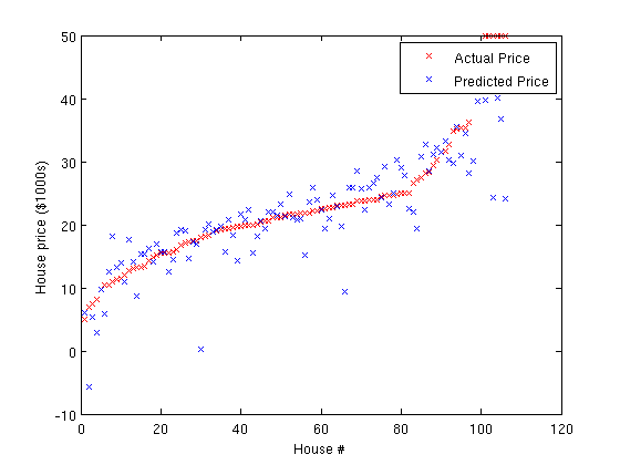
(Yours may look slightly different depending on the random choice of training and testing sets.) Typical values for the RMS training and testing error are between 4.5 and 5.